Inverse problems arise in scientific applications such as biomedical imaging, computer graphics, computational biology, and geophysics, and computing accurate solutions to inverse problems can be both mathematically and computationally challenging.
Assume that
![]() and
and
![]() are given, then a linear inverse problem can be
written as
are given, then a linear inverse problem can be
written as
In this work, we are interested in finding a low rank optimal
regularized inverse matrix
![]() that gives a small reconstruction error. That is,
that gives a small reconstruction error. That is,
![]() should be small for some given error measure
should be small for some given error measure
![]() , e.g.,
, e.g.,
![]() . The particular choice of
. The particular choice of ![]()
![]() and
and
![]() determine the regularization matrix
determine the regularization matrix
![]() . Notice that once
. Notice that once
![]() is found we can efficiently compute
is found we can efficiently compute
![]() by simple
matrix-vector multiplication
by simple
matrix-vector multiplication
![]() . Our
approach is especially suitable for large scale problems
where (1) is solved repeatedly for various
. Our
approach is especially suitable for large scale problems
where (1) is solved repeatedly for various ![]() .
.
In this talk, we focus on efficient approaches to numerical compute
optimal low-rank regularized inverse matrices. In real-life applications,
probability distributions
![]() and
and
![]() are typically not known explicitly.
However, in many applications, calibration or training data are readily
available, and this data can be used to compute a good regularization
matrix.
Let
are typically not known explicitly.
However, in many applications, calibration or training data are readily
available, and this data can be used to compute a good regularization
matrix.
Let
![]() for
for
![]() , where
, where
![]() and
and
![]() are
independently drawn from the corresponding probability distributions.
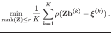
Then the goal is to solve the empirical Bayes risk minimization
problem,
are
independently drawn from the corresponding probability distributions.
Then the goal is to solve the empirical Bayes risk minimization
problem,