We propose a fast iterative solver for large-scale PDE-based nonlinear inverse problems, where measurements are used to reconstruct the spatial variation of parameters. Our motivation is transient hydraulic tomography, which is a method to estimate hydraulic parameters related to the subsurface from pressure measurements obtained by a series of pumping tests. Standard approaches for solving the inverse problem require repeated construction of the Jacobian, which represents the sensitivity of the measurements to the unknown parameters. This is prohibitively expensive because it requires repeated solutions of time-dependent parabolic partial differential equations corresponding to multiple sources and receivers. Additionally, solving the differential equations by time-stepping methods requires computing and storing the entire time history. We use a Laplace Transform-based exponential time integrator to independently compute the solution at multiple times, thus reducing the computational cost.
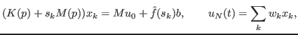
The governing equations for the parabolic PDEs are
where
where
![]() denotes the Laplace Transform of
denotes the Laplace Transform of ![]() ,
, ![]() is
the initial condition and
is
the initial condition and ![]() ,
, ![]() are the
are the ![]() quadrature nodes and
weights respectively, chosen corresponding to the modified Talbot
contour. The approximate solution at a given time can thus be computed
without computing the entire time history. However, solving the shifted
sytem of equations can be computationally expensive for large-scale
problems.
quadrature nodes and
weights respectively, chosen corresponding to the modified Talbot
contour. The approximate solution at a given time can thus be computed
without computing the entire time history. However, solving the shifted
sytem of equations can be computationally expensive for large-scale
problems.
Krylov subspace methods are particularly attractive to solve these
shifted systems of equations (1) because the
shift-invariance property of Krylov subspaces allows us to build a single
solution space across all shifts and an approximate solution for each
shift is then obtained by projecting into a smaller subspace. A single
preconditioner of the form ![]() , for an appropriately chosen
, for an appropriately chosen
![]() , does not successfully precondition all the systems when the range
of values of
, does not successfully precondition all the systems when the range
of values of ![]() is large. We consider a flexible Arnoldi algorithm for
shifted systems that employs multiple preconditioners of the form
is large. We consider a flexible Arnoldi algorithm for
shifted systems that employs multiple preconditioners of the form
![]() for
for
![]() . Changing the preconditioner at each
iteration allows for better preconditioning of the shifted system across
the entire range of shifts.
. Changing the preconditioner at each
iteration allows for better preconditioning of the shifted system across
the entire range of shifts.
The performance of our algorithm will be demonstrated on some challenging synthetic examples of large-scale inverse problems arising from transient hydraulic tomography. We demonstrate that the Krylov subspace accelerated Laplace Transform solver provides a significantly cheaper alternative to time-stepping based solvers.