Finite differences are well-established numerical methods for solving differential equations, but they were limited to structured meshes. The generalized finite differences (GFDs) extend the classical finite differences to unstructured meshes with high-order accuracy. In this paper, we propose a GFD method for elliptic PDEs, and tightly integrate it with a multigrid solver. We refer to this integrated approach as multigrid GFD. Specifically, our method discretizes the PDE and the boundary conditions using GFD to obtain a sparse linear system
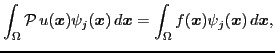
We develop GFD methods based on a weighted least squares (WLS) formulation locally over a weighted stencil at each point, which generalizes the classical interpolation-based finite differences. We have shown recently that the WLS can deliver the same order of accuracy as the interpolation-based approximations, while delivering superior stability, flexibility, and robustness for multivariate approximations over irregular unstructured meshes. The GFD method for PDEs is formulated as follows. Consider a general form of linear, time-independent partial differential equations
To construct the geometric multigrid GFD, which is the core of our
multigrid GFD approach, we derive the restriction and prolongation
operators rigorously for hierarchical meshes. Specifically, let
![]() denote the set of basis functions on the
denote the set of basis functions on the ![]() th finest mesh, and let
th finest mesh, and let
![]() denote the Dirac delta functions on the
denote the Dirac delta functions on the ![]() th finest
mesh. Let
th finest
mesh. Let
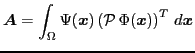
![]() denote the coefficient matrix at the
denote the coefficient matrix at the ![]() th
level, i.e.,
th
level, i.e.,
![]() In a two-level setting, let
In a two-level setting, let
![]() denote a restriction
matrix of the functional space such that
denote a restriction
matrix of the functional space such that
![]() ,
where
,
where
![]() with
with
![]() . Similarly,
. Similarly,
![]() for
for
![]() . We
show that the restriction matrix
. We
show that the restriction matrix ![]() and the prolongation matrix
and the prolongation matrix
![]() in a two-grid method are
in a two-grid method are
In this work, we also investigate the convergence properties of the multigrid solver for the GFDs of elliptic PDEs. We show the multigrid solver may fail to converge for high-order GFD discretizations when using Jacobi or Gauss-Seidel iterations as smoothers. To overcome this issue, we propose new weighting schemes for WLS to improve the diagonal dominance of the linear system from the GFD, and also adopt a damped Gauss-Seidel iteration to enable more robust convergence of multigrid methods. We present the derivations and the numerical experimentations of our method for a number of test problems with various boundary conditions.