Milan Kucharik
Application of JFNK to Kinetic Energy Conservative Remapping of the Nodal Velocity in ALE

T-05 MS B284
Los Alamos National Laboratory
Los Alamos
NM 87545 USA
kucharik@lanl.gov
Markus Berndt
Mikhail Shashkov

Arbitrary Lagrangian-Eulerian (ALE) methods appear to be reasonable compromise between Lagrangian and Eulerian approaches, allowing to solve large variety of fluid problems. The standard ALE algorithm uses a Lagrangian solver to update fluid quantities and the computational mesh in the next time step, which can eventually tangle the mesh. To avoid such problems, mesh regularization (untangling or smoothing) is applied in the case of low mesh quality, followed by a remapping step that interpolates all fluid quantities from the Lagrangian to the smoothed mesh.

Here, we focus on the last part of the ALE algorithm - remapping - in the case of a staggered discretization, where scalar quantities (density, pressure, specific internal energy) are defined inside mesh cells, and vector quantities (positions, velocities) are defined on mesh nodes. A staggered discretization is used in most current ALE codes. Generally, remapped nodal kinetic energy is not equal to nodal kinetic energy obtained from remapped velocities, and this discrepancy leads to energy conservation violation and consequently to wrong shock speeds. The kinetic energy discrepancy is usually treated by distributing it to the internal energy of adjacent cells [2].

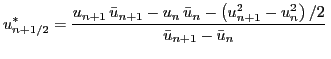
An alternative 1D approach introduced in [1] is based on the construction of high-order interpolated velocities $u^*_{n+1/2}$ used for momentum fluxes (and thus for the velocity update)

$$\tilde{m}_{n}\, \tilde{u}_{n} = m_n\, u_n + F^{m}_{n,n+1/2}\, u^*_{n+1/2} - F^{m}_{n,n-1/2}\, u^*_{n-1/2}$$ (1)

such that the kinetic energy discrepancy is automatically eliminated. Here, $F^{m}_{n,n\pm 1/2}$ stands for mass fluxes around node $n$, which are also used for the nodal mass update in a similar flux form

$$\tilde{m}_{n} = m_n + F^{m}_{n,n+1/2} - F^{m}_{n,n-1/2} \,$$ (2)

This method expresses the new kinetic energy $\tilde{K}$ in each node in a flux form

$$\tilde{K}_{n} = K_n + F^{K}_{n,n+1/2} - F^{K}_{n,n-1/2} \,$$ (3)

where fluxes $F^{K}$ can be computed from known quantities and unknown inter-nodal flux velocities $u^*_{n \pm 1/2}$. To achieve energy conservation, there must be an unique flux between every two nodes:

$$F^{K}_{n,n+1/2} = F^{K}_{n+1,n+1/2} \equiv F^{K}_{n+1/2} \, \,\, \forall n \,$$ (4)

After substituting for all $F^{K}$, we obtain a system of coupled quadratic equations for all $u^*$,

$$u^{*}_{n+1/2} = \frac{ u_{n+1}\, \bar{u}_{n+1} - u_{n} \, \bar{u}_{n} - \left(u_{n+1}^2-u_{n}^2\right)/2} {\bar{u}_{n+1} - \bar{u}_{n}} \,$$ (5)

where $\bar{u}_n = (u_n + \tilde{u}_n)/2$, and the new velocities $\tilde{u}_n$ are defined in (1). This system can either be solved with a fixed point iteration, or with a Newton solver.

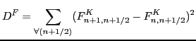
In this presentation, we demonstrate that the system (5) does not always have a solution, and analyze this situation. Two alternative approaches will be introduced.

In the first approach, the flux equality (4) is not enforced strictly, but its discrepancy is minimized in a least squares sense

$$D^{F} = \sum\limits_{\forall (n+1/2)} (F^{K}_{n+1,n+1/2} - F^{K}_{n,n+1/2})^2$$ (6)

by differentiating $D^{F}$ with respect to all $u^*$ and solving a system $\partial D^F / \partial u^*_{n+1/2} = 0$ for all $n+1/2$. Thus, the kinetic energy discrepancy is minimized as much as possible, but is not guaranteed to equal zero.

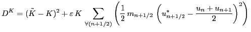
In the second approach, the kinetic energy discrepancy is directly minimized. Unfortunately, zero kinetic energy discrepancy is generally satisfied by infinitely many solutions. Because flux velocities $u^*_{n+1/2}$ represent values interpolated from adjacent nodal velocities $u_{n}$ and $u_{n+1}$, this velocity should remain bounded by these neighbor values and no under/overshoots should appear. Thus, additional terms are added to the kinetic energy discrepancy formula, which enforce these bounds during minimization

$$D^{K} = (\tilde{K} - K)^2 + \varepsilon\, K\, \sum\limits_{\foral... ...m_{n+1/2}\, \left( u^*_{n+1/2} - \frac{u_{n} + u_{n+1}}{2} \right)^2 \right) \,$$ (7)

Similarly to our first approach, the minimization is done by solving a system $\partial D^K / \partial u^*_{n+1/2} = 0$ for all $n+1/2$. This approach finds a zero discrepancy solution that is generally different from the solution of system (4) (if it exists). In both approaches (6) and (7), the Jacobian-free Newton-Krylov solver [3] with a possible preconditioning is used.

We will also mention a generalization of these approaches to 2D logically orthogonal meshes (including corner coupling), and demonstrate their behavior in the context of an ALE hydro code for a particular fluid flow problem.