Error analysis of BDF Compound-Fast multirate method for
differential-algebraic equations
Arie A. Verhoeven
HG 8.47 (Technische Universiteit Eindhoven)
Den Dolech 2, 5600 MB Eindhoven, The Netherlands
averhoev@win.tue.nl
Jan ter Maten, Bob Mattheij, Theo Beelen,
Ahmed El Guennouni, Bratislav Tasic
Analogue electrical circuits are usually modeled by
differential-algebraic equations (DAE) of type:
where
 represents the state of
the circuit. A common analysis is the transient analysis,
which computes the solution
represents the state of
the circuit. A common analysis is the transient analysis,
which computes the solution
 of this
non-linear DAE along the time interval
of this
non-linear DAE along the time interval ![$ [0,T]$](img4.png) for a given
initial state. Often, parts of electrical circuits have
latency or multirate behaviour.
for a given
initial state. Often, parts of electrical circuits have
latency or multirate behaviour.
For a multirate method it
is necessary to partition the variables and equations into
an active (A) and a latent (L) part. The active and latent
parts can be expressed by
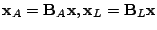 where
where
 are permutation matrices. Then
equation (1) is written as the following
partitioned system:
are permutation matrices. Then
equation (1) is written as the following
partitioned system:
In contradiction to classical
integration methods, multirate methods integrate both parts
with different stepsizes. Besides the coarse time-grid
 with stepsizes
 , also a refined time-grid
 is used with stepsizes
 and multirate factors
  . If the two
time-grids are synchronized,
. If the two
time-grids are synchronized,
 holds for all
  . There are a lot of multirate approaches
for partitioned systems but we will consider the
Compound-Fast version of the BDF methods. This method
performs the following four steps:
. There are a lot of multirate approaches
for partitioned systems but we will consider the
Compound-Fast version of the BDF methods. This method
performs the following four steps:
- The complete system is integrated at the coarse time-grid.
- The latent interface variables are interpolated at the
refined time-grid.
- The active part is integrated at
the refined time-grid, using the interpolated values at the
latent interface.
- The active solution at the coarse
time-grid is updated.
The local
discretization error  of the compound phase still
has the same behaviour
of the compound phase still
has the same behaviour
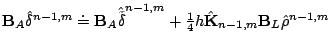
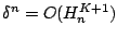 . Let
. Let
 be the Nordsieck
vectors which correspond to the predictor and corrector
polynomials of
be the Nordsieck
vectors which correspond to the predictor and corrector
polynomials of
 . Then the error can
be estimated by
. Then the error can
be estimated by
 :
:
Now
 is
the used weighted error norm, which must satisfy
is
the used weighted error norm, which must satisfy
 TOL
TOL .
.
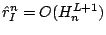
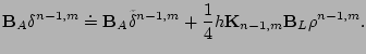
The local discretization error
 is defined as the residue after inserting the exact solution
in the refinement BDF scheme. During the refinement instead
of
the perturbed local error
is defined as the residue after inserting the exact solution
in the refinement BDF scheme. During the refinement instead
of
the perturbed local error
 is estimated. A tedious analysis
yields the following asymptotic behaviour:
Here
is estimated. A tedious analysis
yields the following asymptotic behaviour:
Here
 is the interpolation error at the
refined grid and
is the interpolation error at the
refined grid and
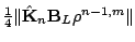
 is the coupling
matrix. The perturbed local discretization error
is the coupling
matrix. The perturbed local discretization error
 behaves as
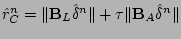
 and can be estimated in a similar way
as . Thus the active error estimate
and can be estimated in a similar way
as . Thus the active error estimate
 satisfies
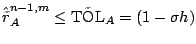
 . Let
. Let
 be the interpolation order, then it can be shown that
 is less than
Here
is less than
Here
 are the Nordsieck
vectors which correspond to the predictor and corrector
polynomials of
are the Nordsieck
vectors which correspond to the predictor and corrector
polynomials of
 . This error estimate
 has the asymptotic behaviour
 . It follows that
 satisfies:
If
satisfies:
If
 TOL
TOL
 TOL
TOL and
and
 TOL then
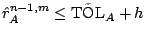 TOL
TOL TOL.
TOL.
We tested a
circuit with
 inverters. The location of the
active part is controlled by the connecting elements and the
voltage sources. The connecting elements were chosen such
that the active part consists of 3 inverters. We did an
Euler Backward Compound-Fast multirate simulation on
inverters. The location of the
active part is controlled by the connecting elements and the
voltage sources. The connecting elements were chosen such
that the active part consists of 3 inverters. We did an
Euler Backward Compound-Fast multirate simulation on
![$ [0,10^{-8}]$](img49.png) with
with
 . We get accurate
results combined with a speedup factor 13.
. We get accurate
results combined with a speedup factor 13.
![$\displaystyle \qquad \qquad \qquad
\frac{d}{dt}\left[
\mathbf{q}(t,\mathbf{x})\right]+
\mathbf{j}(t,\mathbf{x})=\mathbf{0},
\qquad \qquad \qquad (1)
$](img1.png)
![$\displaystyle \hat{\delta}^n = \frac{-H_n}{T_n - T_{n-K-1}} \left
[\bar{\mathbf{Q}}_{1}^{n}-\bar{\mathbf{P}}_{1}^{n} \right ].
$](img20.png)
![$\displaystyle \hat{r}_I^{n} =
\frac{1}{4}\frac{H_n}{T_n - T_{n-L-1}}
\Vert\hat{...
...mathbf{B}_L
\left[\bar{\mathbf{X}}_{1}^n
-\bar{\mathbf{Y}}_{1}^n\right] \Vert.
$](img35.png)