Some modeling and simulations efforts have historically encompassed multiscale phenomena without explicitly handling multiscale features. One such area is density functional theories for inhomogeneous fluids (Fluid-DFTs). In this presentation we look at Fluid-DFTs from a fresh perspective, calling out the fact that Fluid-DFTs incorporate multiple length scales that are introduced in a way such that each longer scale increases the fidelity of the model. By viewing Fluid-DFTs from this perspective, we develop a mathematical framework and a collection of solution algorithms that have a dramatic impact on the robustness, performance and scalability of the implicit equations generated by Fluid-DFTs.
The basic
framework for all of our solver algorithms reflects the
importance of inter-physics coupling in the extended
variable formulation of the
Fluid-DFTs.
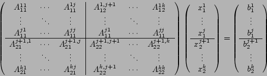
This physics coupling led
us to a physics-based block matrix formulation in order to
partition critical and nonlocal ancillary variables. The
idea is to partition the data into blocks that can be
optimally managed or solved. The general ![]() block
matrix is
block
matrix is
Given this two-level structure, the basic strategy for solving each global linear system generated by Newton's method is as follows:
Given this basic framework, we will describe specific solvers for special categories of Fluid-DFT problems, including 2 and 3 dimensional hard-sphere problems and polymer chains. We give results for several problem areas including nanopore and lipid bi-layer models where this Schur complement approach provides one to two orders of magnitude improvement in performance and an order of magnitude reduction in memory requirements.