Next: About this document ...
Eric de Sturler
Integrated Model Reduction Strategies for Nonlinear Parametric Inversion
Department of Mathematics
Virginia Tech
Blacksburg
VA 24061
sturler@vt.edu
Chris Beattie
Serkan Gugercin
Misha E. Kilmer
We will show how reduced order models can significantly reduce the cost of general
inverse problems approached through parametric level set methods.
Our method drastically reduces the solution of forward problems in diffuse optimal
tomography (DOT) by using interpolatory parametric model reduction.
In the DOT setting, these surrogate models can approximate both the cost functional and
associated Jacobian with little loss of accuracy and significantly reduced cost.
We recover diffusion and absorption coefficients,
 and
and
 , respectively,
using observations,
, respectively,
using observations,
 ,
from illumination by source signals,
,
from illumination by source signals,
 .
We assume that the unknown fields can be characterized by
a finite set of parameters,
.
We assume that the unknown fields can be characterized by
a finite set of parameters,
![$ \mathbf{p}=[p_1,\ldots,\,p_{\ell}]^T$](img5.png) .
Discretization of the underlying PDE gives the following, order
.
Discretization of the underlying PDE gives the following, order  ,
differential algebraic system,
,
differential algebraic system,
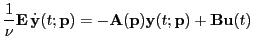 with with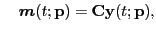 |
(1) |
where
 denotes the discretized photon flux;
![$ \boldsymbol{m}=[m_1,\,\ldots,\, m_{n_{det}}]^T$](img10.png) is the vector of detector outputs;
the columns of
is the vector of detector outputs;
the columns of
 are discretizations of the source ``footprints"; and
 is the discretization of the diffusion and
absorption terms, inheriting
the parameterizations of these fields.
is the discretization of the diffusion and
absorption terms, inheriting
the parameterizations of these fields.
Let
 ,
,
 , and
, and
 denote Fourier transforms of
 ,
, and
,
, and
 , respectively.
Taking the Fourier transform of (
, respectively.
Taking the Fourier transform of (![[*]](file:/usr/share/latex2html/icons/crossref.png) ), we find
), we find
 where where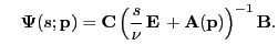 |
(2) |
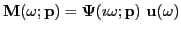
 is a mapping from sources (inputs) to
measurements (outputs)
in the frequency domain; it is the transfer function of the dynamical system
().
Given a parameter vector,
is a mapping from sources (inputs) to
measurements (outputs)
in the frequency domain; it is the transfer function of the dynamical system
().
Given a parameter vector,
 , and absorption field,
 ,
input source,
,
input source,
 , and frequency
  ,
,
 denotes
the vector of observations predicted by the forward model.
For
denotes
the vector of observations predicted by the forward model.
For  sources and
 frequencies, we get
which is a vector of dimension
 .
We obtain the empirical data vector,
.
We obtain the empirical data vector,
 , from actual observations, and solve the optimization problem:
The computational cost of evaluating
 is dominated
by the solution of the large, sparse block linear systems in ()
for all frequencies
.
is dominated
by the solution of the large, sparse block linear systems in ()
for all frequencies
.
To reduce costs while maintaining accuracy, we seek a much smaller
dynamical system of order  that replicates the input-output map of ():
 with with |
(3) |
where the new state vector
 ,
,
 ,
,
 , and
, and
 such that
 .
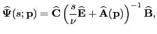
The surrogate transfer function is
.
The surrogate transfer function is
which requires only the solution of linear systems
of dimension
; hence drastically reducing the cost.
For a given parameter value
 used in an optimization step,
a reduced (surrogate) model for the necessary function evaluations
at the frequency
, involves the construction of a reduced parametric model
of the form ()
with transfer function
used in an optimization step,
a reduced (surrogate) model for the necessary function evaluations
at the frequency
, involves the construction of a reduced parametric model
of the form ()
with transfer function
 that satisfies
 |
(4) |
This is exactly what interpolatory model reduction achieves.
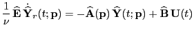
Moreover, the transfer function
 of the
reduced-model also satisfies
of the
reduced-model also satisfies
 and and  |
|
|
|
The use of interpolatory projections allows us to match both function and
gradient values exactly
without computing them, requiring instead only that
the computed projection spaces defining the reduced model
contain particular (stably computable) vectors.
If we were to compute a reduced-model for every
parameter point
and frequency
,
and use these
reduced-models in the forward model,
the solution of the inverse problem would proceed in exactly the same way
as in the case of the full-order forward model -
the nonlinear optimization algorithm would not see the difference between the
full and reduced forward problems.
Of course, computing a new surrogate-model for every parameter value is infeasible.
Hence, we focus on methods of constructing surrogate-models that have
high-fidelity over a wide range of parameter values and consider effective
approaches for updating the surrogate models. We will present numerical
examples that illustrate the effectiveness of these methods.
Next: About this document ...
root
2012-02-20