


Next: About this document ...
Aleksandar Jemcov
Application of Vector Sequence Extrapolation to Iterative Algorithms in Computational Fluid Dynamics
10 Cavendish Court
Lebanon
NH
03766
USA
aj@fluent.com
Joseph P. Maruszewski
The vector extrapolation methods are the generalization of the
Aitken's
 method for the scalar equations that allow
a significant acceleration of the monotonic convergence. The idea
of the convergence acceleration through the extrapolation methods
is based on the transformation of a slowly converging sequence
method for the scalar equations that allow
a significant acceleration of the monotonic convergence. The idea
of the convergence acceleration through the extrapolation methods
is based on the transformation of a slowly converging sequence
 into a new sequence
  converging to the same
limit faster than the initial one. The transformation
converging to the same
limit faster than the initial one. The transformation
 |
(1) |
is constructed by interpolating a finite number of terms in the
sequence , thus effectively computing the sequence limit
through the following linear combination:
 |
(2) |
The vector extrapolation methods extend this approach to the
sequences whose elements are vectors in the same way they were
used in Eq. (![[*]](file:/usr/share/latex2html/icons/crossref.png) ) to accelerate the scalar sequences.
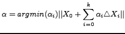
Weighting coefficients
) to accelerate the scalar sequences.
Weighting coefficients  are determined by minimizing
the error terms defined as the difference between the limit of
the sequence
are determined by minimizing
the error terms defined as the difference between the limit of
the sequence  and the arbitrary elements of the sequence
 :
:
 |
(3) |
For the linear fixed-point functions this is achieved by
observing that the initial error
 can be related to
the subsequent error
can be related to
the subsequent error
 through the powers of the
iteration matrix of the fixed-point function:
through the powers of the
iteration matrix of the fixed-point function:
 |
(4) |
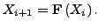
Here the fixed point function is defined by
 |
(5) |
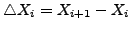
If we take the definition of the error, Eq. () and
observing that the arbitrary element of the sequence can be
expressed as
 |
(6) |
and if we substitute Eq. (), we can arrive to the
conditions that the weighting coefficients must satisfy in order
to minimize the error in Eq. ():
 |
(7) |
Eq. () is equivalent to the following constrained
minimization problem:
 |
(8) |
such that
 |
(9) |
Here
 .
In other words, Eq. () corresponds to finding the
coefficients of the minimal polynomial associated with the
iteration matrix
.
In other words, Eq. () corresponds to finding the
coefficients of the minimal polynomial associated with the
iteration matrix  and this indicates an intimate link
between vector sequence extrapolation and Krylov subspace
methods. Another point of view that we will be taking here is
that the vector sequence extrapolation methods correspond to the
preconditioned Krylov subspace methods that use the fixed-point
algorithms as the nonlinear preconditioners.
and this indicates an intimate link
between vector sequence extrapolation and Krylov subspace
methods. Another point of view that we will be taking here is
that the vector sequence extrapolation methods correspond to the
preconditioned Krylov subspace methods that use the fixed-point
algorithms as the nonlinear preconditioners.
Strictly speaking, Eq. () is valid for the linear fixed
point functions but the method can be extended to the nonlinear
fixed point functions through a local linearization and by the
inclusion of restarts in the algorithm. The general form of
the nonlinear fixed-point functions considered here takes the
following form:
 |
(10) |
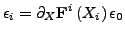
Using the local linearization, the initial and  -th error are
related through the powers of the Jacobian of the fixed point
function with the second order accuracy, similarly to
Eq. ():
-th error are
related through the powers of the Jacobian of the fixed point
function with the second order accuracy, similarly to
Eq. ():
 |
(11) |
The nonlinearly preconditioned Krylov subspace method algorithm
can be devised that is similar to the algorithm described in
Eq. () and Eq. () but with the use of
restarts.
The vector extrapolation method is applied to problems in
Computational Fluid Dynamics and it is shown that it leads to a
significant acceleration of the convergence rates. Moreover, the
method can be applied to the acceleration of any fixed-point
algorithm with the minimal or no changes to the original
algorithm. Results are demonstrated for the cases of the
compressible and incompressible flows as well in conjunction with
the explicit and implicit algorithms.
Next: About this document ...
Marian
2008-02-26